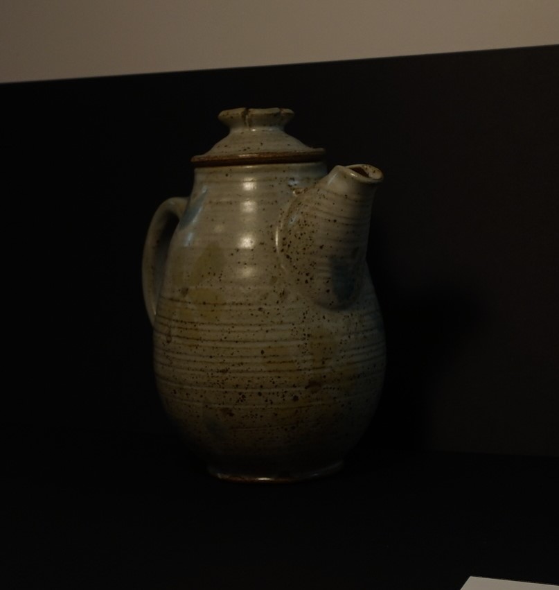
The goal of this project is to take a set of 2D images of a given object, taken from two stationary cameras, and create a 3D model of the item. A checkerboard with given dimensions has been photographed by both cameras throughout the scene to provide reference points for camera calibration.
After these parameters are set, the goal is to decode the structured light images taken of the object. From the point clouds generated, meshes can be cleaned and stitched together to produce the final 3D object.
Various techniques will be used along the way to clean up the mesh in order to produce a model which highly resembles the initial object.
The calibration script utilizes the intrinsic parameters provided by the photographer. However, the extrinsic properties are yet to have been found. The calibration algorithm is fed these intrinsic parameters along with a calibration image. The image is loaded, and the corners are detected using the Harris Corner Detector. The user is expected to click on corners in a specified order.
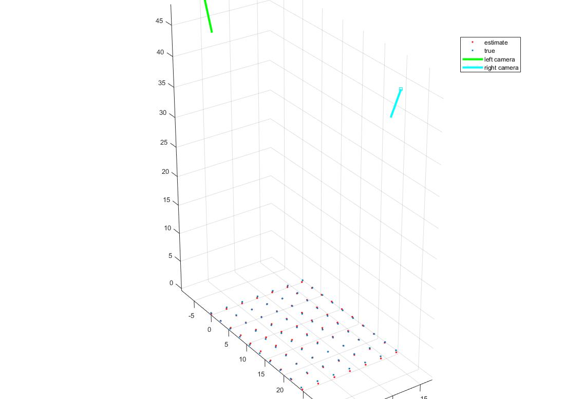
After initial extrinsic parameters are set, the algorithm optimizes these parameters over the rotation and translation variables (focal point and principle offset are fixed). The provided function ‘lsqnonlin’ solves the nonlinear least-squares by finding a set of parameters that minimizes the total error between the given 3D points projected through the camera in 2D with varied settings and the given 2D points while attempting to avoid settling at local minima. After the function has minimized the error in the parameters, the camera’s extrinsic properties are set and returned along with the 2D point set from the grid, and the estimated 3D point set from the triangulation of the two cameras with the optimized parameters.
First, the camera parameters are loaded into the function for use with decoding. The structured light images are then fed to the decode algorithm which produce a 3D mesh. This is done by assigning a unique gray code to each pixel in the scene according to whether it falls in the light or out of the light in each image in the set. The gray code is then converted to decimal and compared to the decimal values in the corresponding camera’s image.
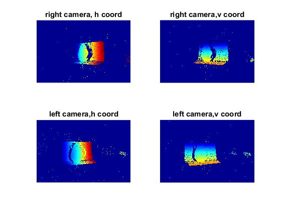
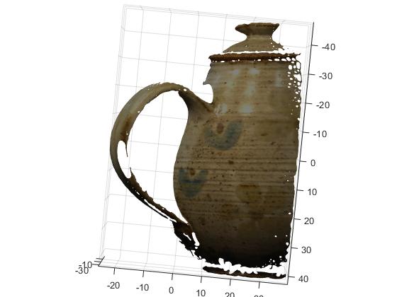
If a correspondence is found, a 3D point is set. All points without correspondences are not considered in the 3D mesh and are subsequently not included in the 3D color buffer. This buffer takes the corresponding 2D points from the RGB reference images, averages them, and assigns the resulting value to its matching 3D point. Now that we have the corresponding 2D point sets, color values, and camera parameters, a 3D point cloud can be constructed by triangulating the sets through the cameras. This 3D cloud is saved for later use.
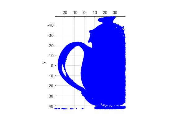
The clean mesh algorithm iterates through each set of 3D point clouds. The center of mass for each cloud is calculated, and then translated to the origin. From here, a bounding box is set; this cuts off any point values above or below specified threshold values in the x, y, and z directions. These points are not only removed from the 3D point set, but also from the 2D point set and the 3D color buffer for later use with Delaunay triangulation.
Each partially cleaned mesh is loaded into the function. After the thresholds for max point location error and max edge lengths are set, the algorithm proceeds to utilize the ‘nbr_error’ function. This provided algorithm projects each 2D point set in 3D, and compares its value to the median of its nearest neighbors. The difference of the two locations is saved as the error for that pixel. Any pixels whose error exceeds the user defined threshold is dropped from the 2D and 3D point sets.
Next, the provided ‘tri_error’ function is executed on the set of points. This function performs Delaunay triangulation on the set of points, computes each triangles longest edge, and assigns this as the error for said triangle. The set of triangles are then exported to the main function with their respective errors. Then, each triangle with an error greater than the defined threshold is pruned from the set. Lastly, the provided ‘nbr_smooth’ function smooths the mesh by taking each 3D point and moving it to the mean location of its neighbors. This final cleaned mesh is exported as a ‘.ply’ file using the provided function ‘mesh_2_ply’.
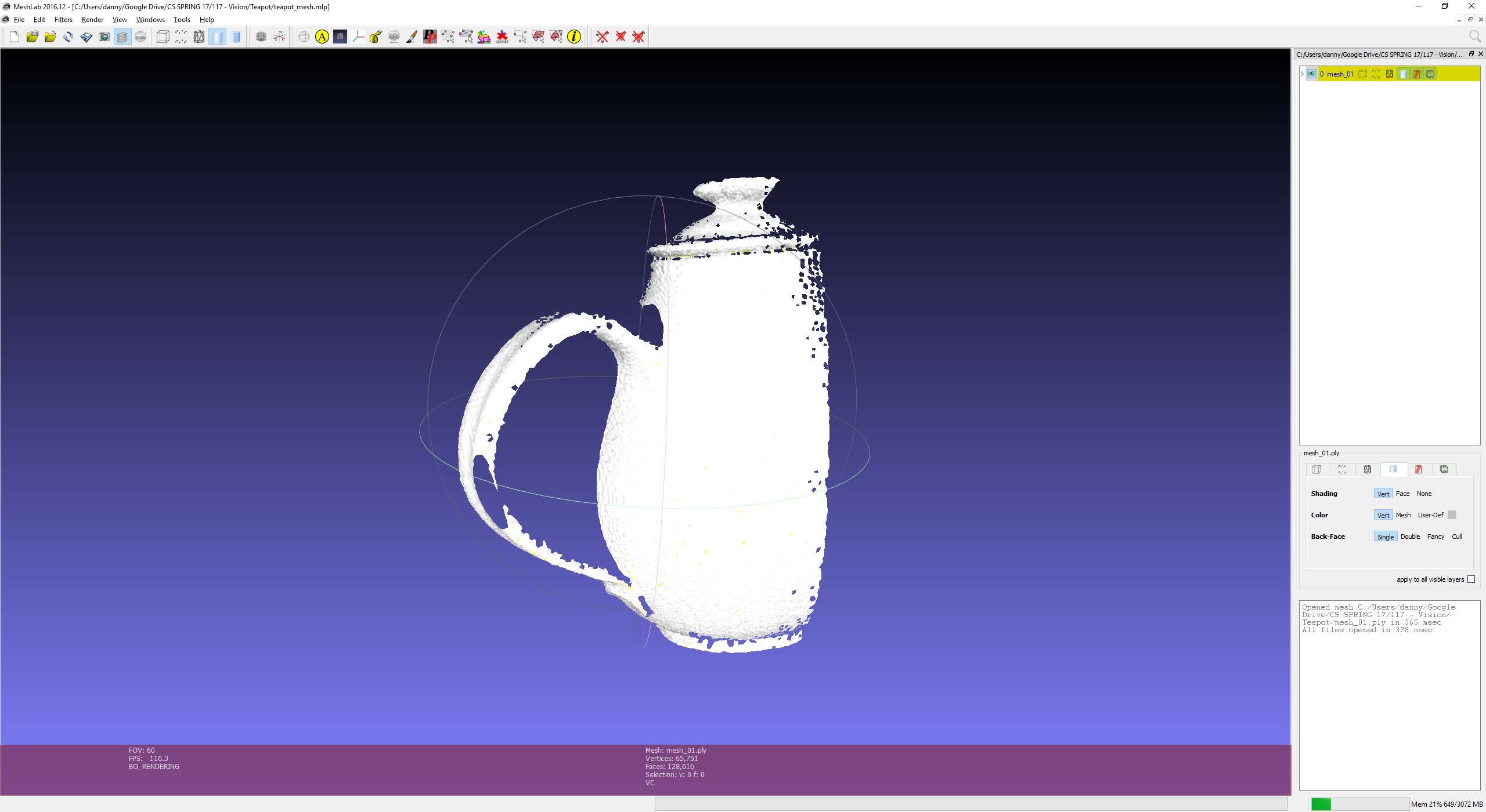
The individual meshes are then loaded into Meshlab for alignment. The user is required to set the initial points for Meshlab to run its iterative closest point (ICP) alignment algorithm. This works by overlaying the meshes in an initial configuration set by the user, and modifying its location in an attempt to minimize the difference in distances between both point clouds. Once Meshlab has finished with the ICP and all meshes have been aligned, the mesh is flattened and exported as a ‘.ply’ file.
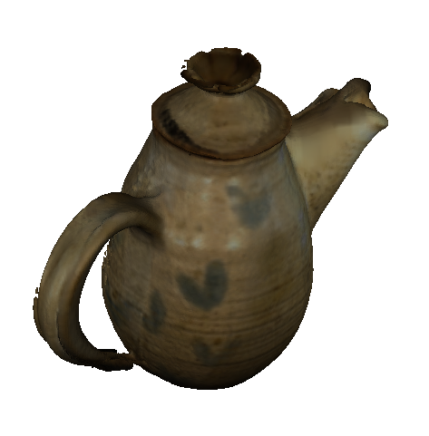
The final step is to create a closed mesh using the ‘Screened Poisson Surface Reconstruction’. This provided executable takes in the aligned ‘.ply’ file and returns a closed surface. It does this by breaking down the problem into a Poisson problem; it computes the indicator function, and the divergence, and extracts the iso- surface.
The results of the pipeline were a success. That being said, this is not an easy task for a computer algorithm to solve. The reason for this is that a lot of human interaction is required to create a mesh that is this clean.
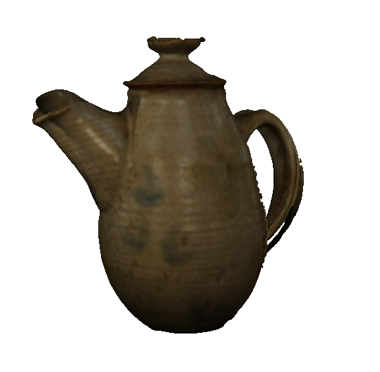
For example, without the bounding box to cleanup the point cloud, or the Meshlab interactive alignment, the pipeline wouldn’t have been effective. These can certainly be considered limitations. The success comes from the ability to create a closed, clean surface that highly resembles the source image.
Overall, I think that the pipeline works well for basic reconstruction, but some extra features would be welcome in order to produce superior models.