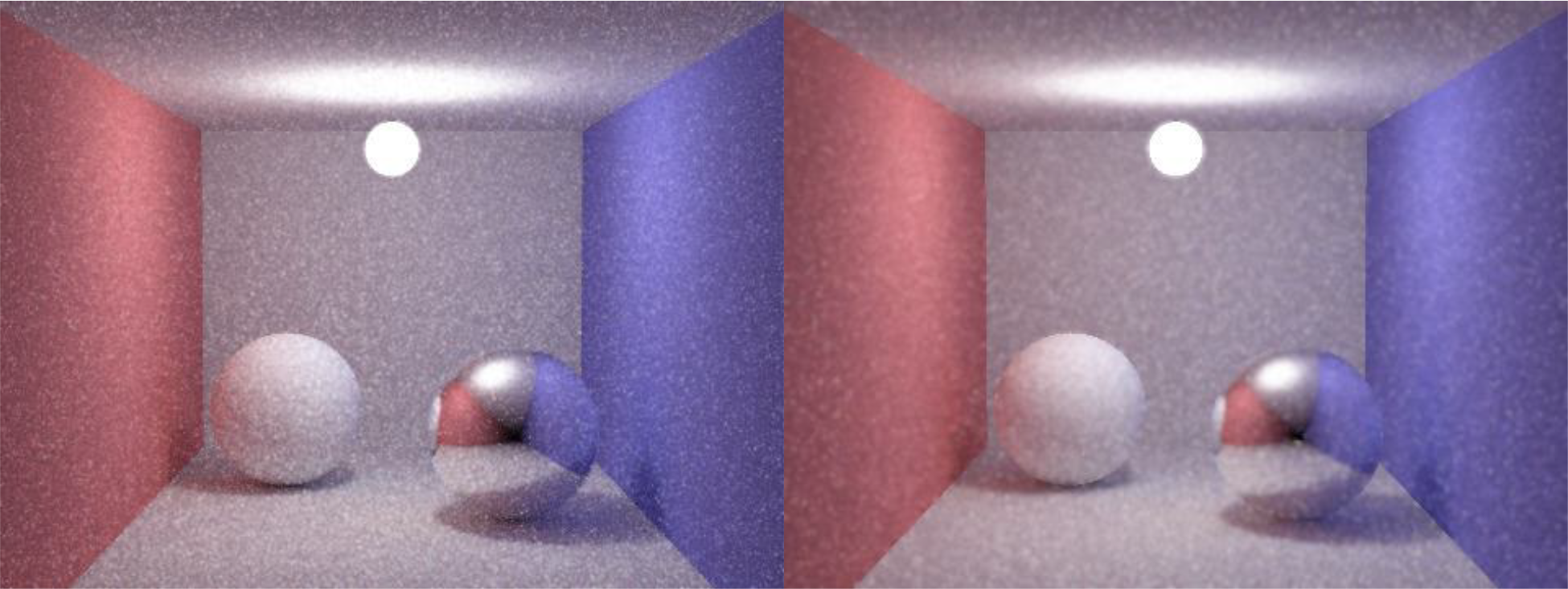
Monte Carlo ray tracing utilizes random point sampling, and estimated integrals to produce highly realistic images. However, the drawback is that the algorithm needs to take upwards of 1024 samples per pixel to obtain an image with acceptable noise levels. As one would imagine, this is extremely time consuming.
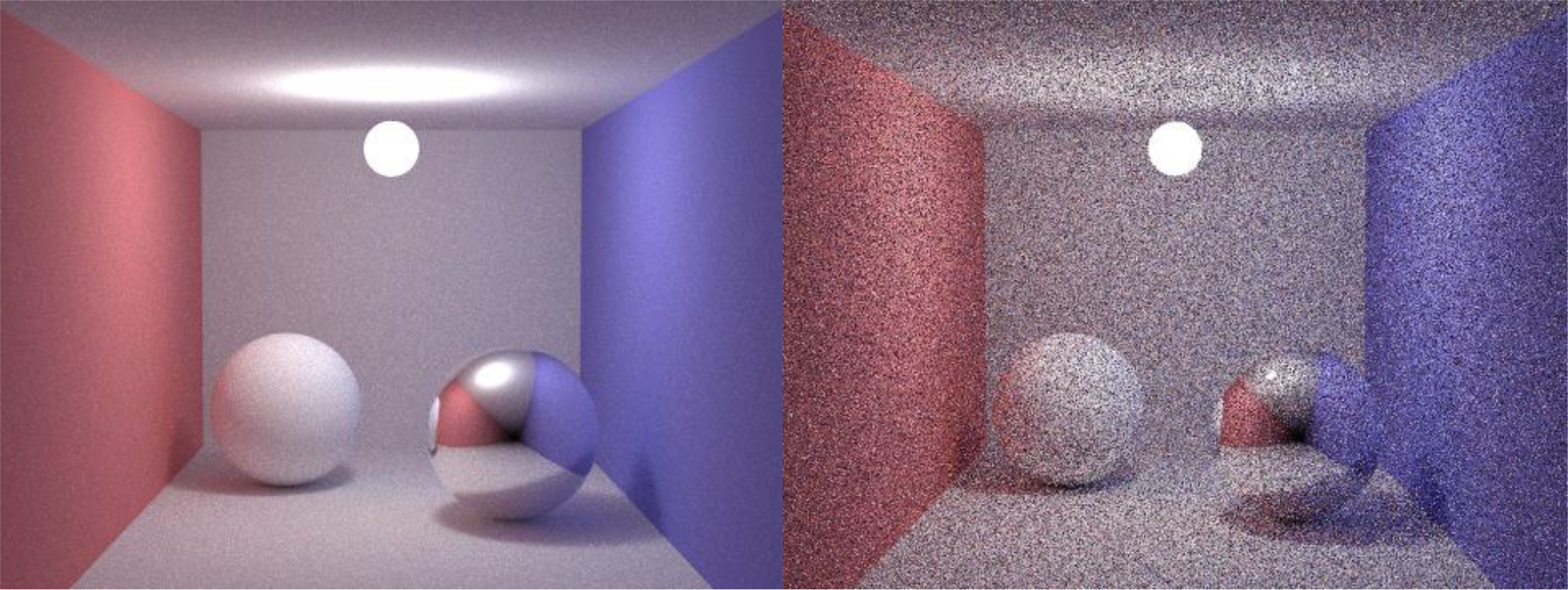
This being said, a number of post processing techniques can be used to drastically reduce the noise while maintaining the detail of the scene that Monte Carlo renderings are known for.
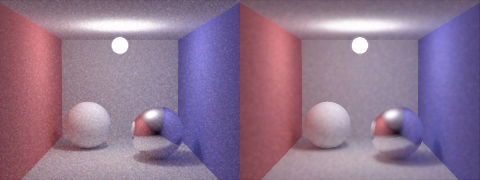
As an initial attempt at reducing the noise, I implemented three simple filters which only take a pixel’s color value into consideration. These filters take as input a vector containing the pixel values, the height and width of the image, and the size of the kernel to be used.
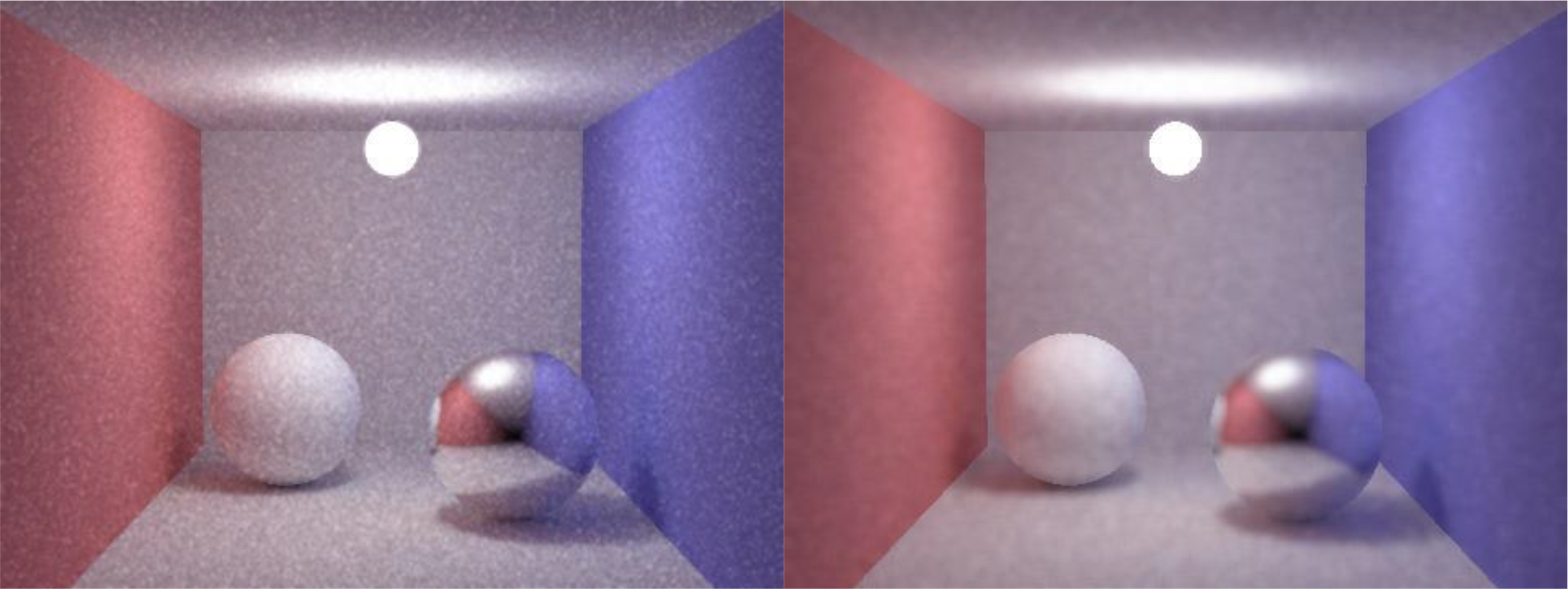
The first is the simple mean filter. This function takes a neighborhood around a given pixel, averages all the values, and applies it to the center pixel. The overall effect of this filter is a blurring effect which is effective at reducing noise, but at the expense of overall detail.
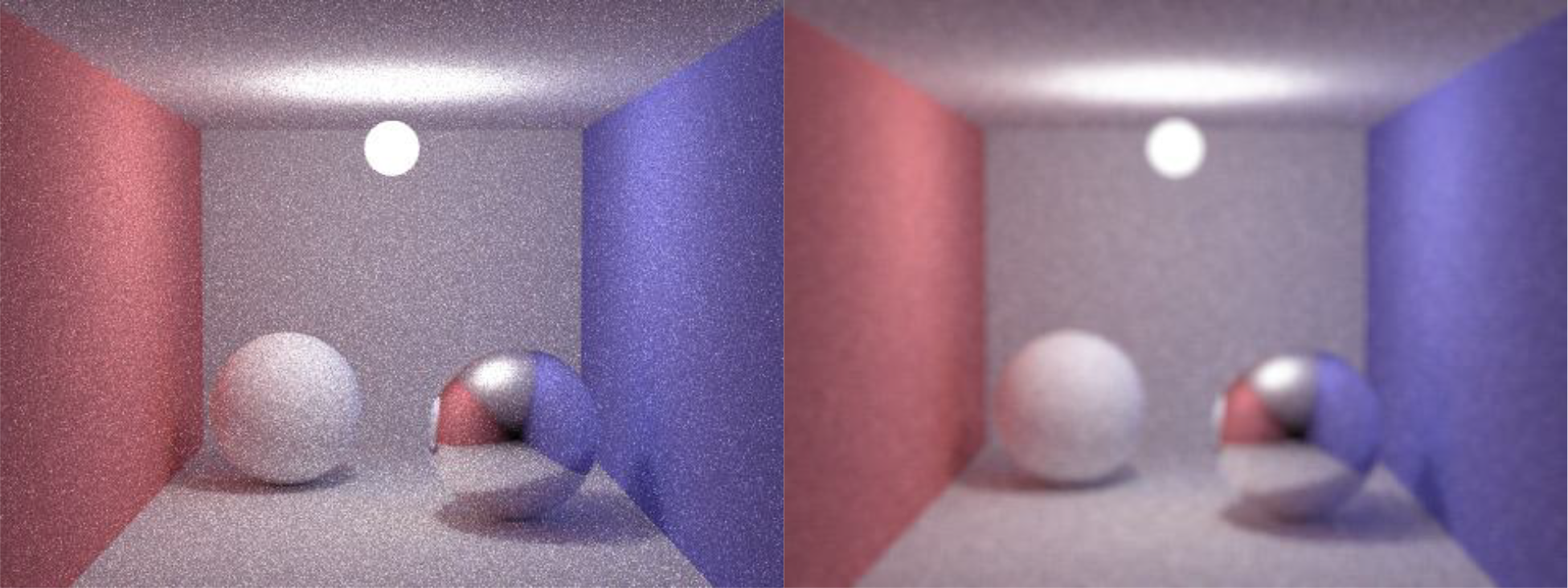
The second filter is the simple median filter. The median filter, in principle is great at reducing periodic noise and less great at reducing aperiodic noise. This function takes the median of the neighbors surrounding a pixel and applies it to said pixel. This filter reduced some noise, but not nearly enough to be acceptable on its own.
The third and last of the simple filters is the simple gaussian. This function takes the size of the kernel inputted by the user and generates a gaussian kernel (Pascal’s triangle). After generating the kernel, the algorithm applies it to the neighborhood around a given pixel. The surrounding pixels are multiplied by the weights supplied by the kernel and added together. The total is the divided by the sum of the numbers in the kernel.
The main idea is to obtain a weighted average of pixels giving the pixels nearest to the center the most weight and reduce as the pixels get further away. This filter had the effect of reducing noise, but also at the expense of reducing image fidelity overall.
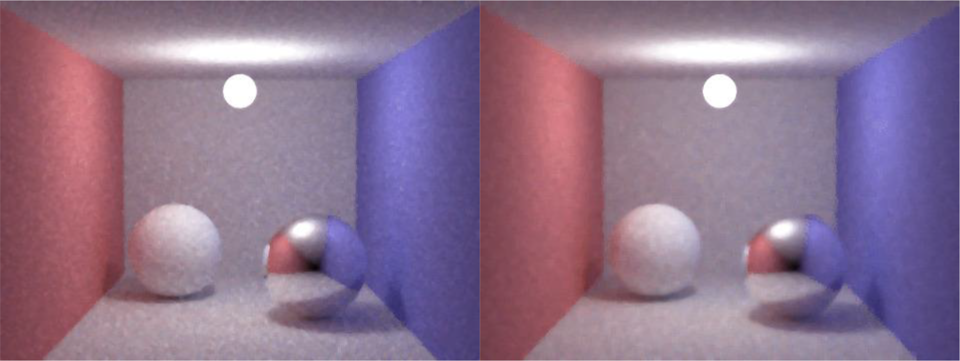
The simple filters worked well enough for a preliminary trial, but they were not making use of all of the information that the scene has to offer. These filters were blurring across the entire image without taking into concern which pixels belonged to which object. This led me to implement a series of filters which considered the objects that each pixel belonged to.
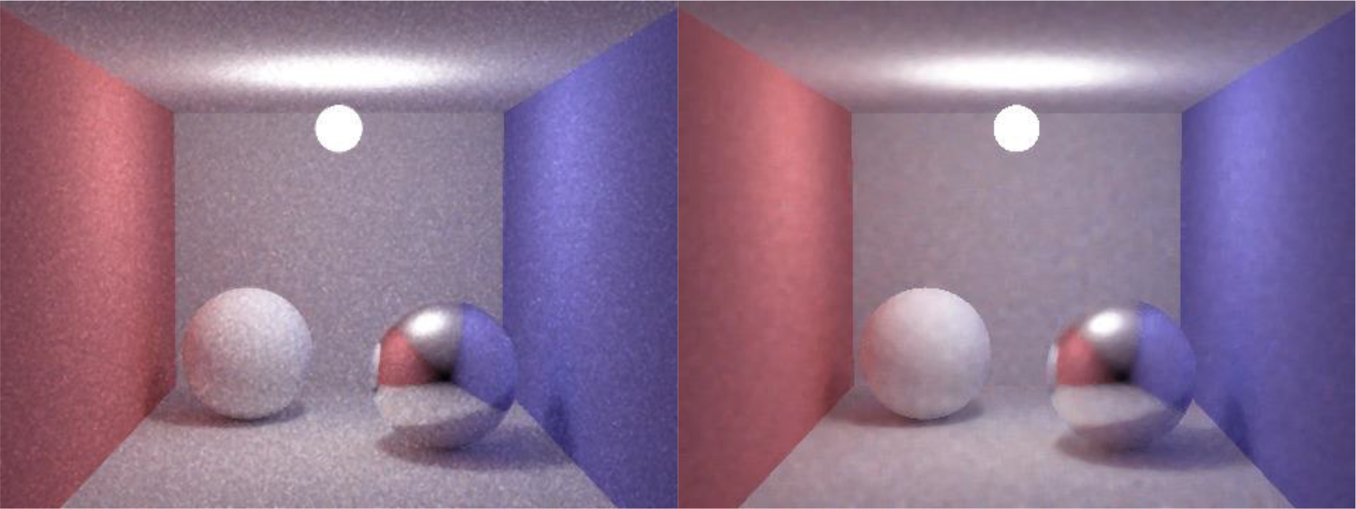
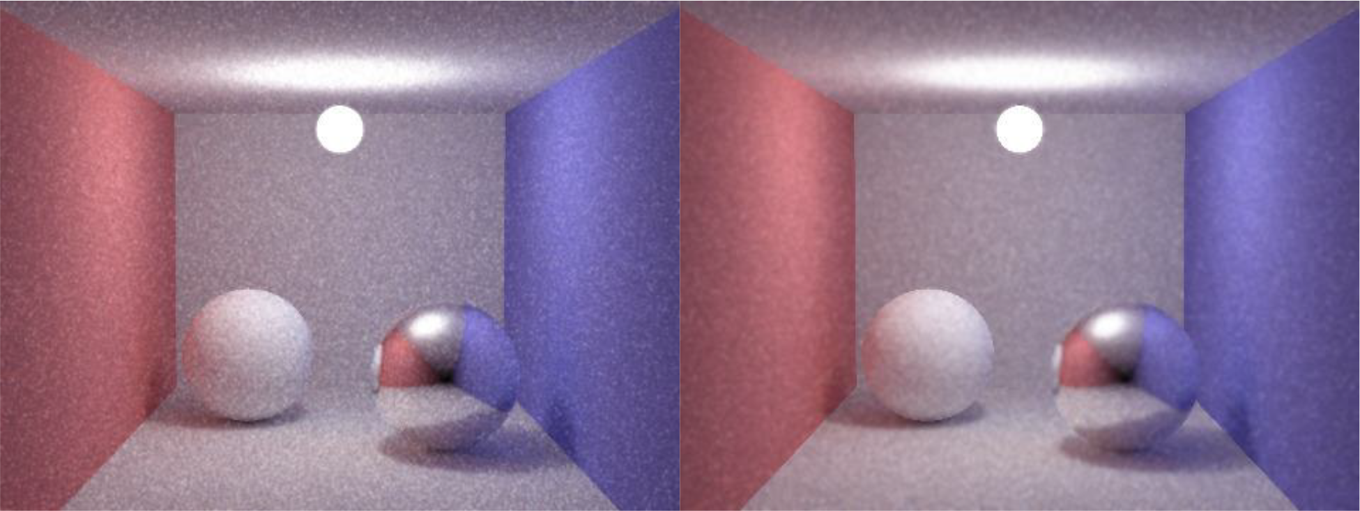
The first of the series is the object mean which takes the neighboring pixels and averages them together. However, the algorithm only considers any neighbor a viable candidate if it shares the same object as the center pixel. This filter was a big improvement on the simple mean filter as it helped to preserve hard edges along object boundaries.
The second object filter is the object median. This filter takes the neighboring pixels, finds those pixels which share the same object, takes the median value of the group, and assigns it to the center pixel. This method was able to reduce a significant amount of noise while preserving the high frequency detail of the scene.
The last object based method is the object based gaussian filter. This filter took the user inputted size and constructed a gaussian kernel to be applied across the image. It then took each pixel, considered pixels with the same object as the center pixel, applied the weight according to the gaussian kernel, computed the sum of those weighted values, and divided by only those weights which contributed to the total.
This weighted average was then applied to the center pixel. This filter gives precedence to pixels closer to the center pixel while still considering only those pixels which share the same object. The results obtained from this filter were acceptable and greatly reduced noise throughout the image.
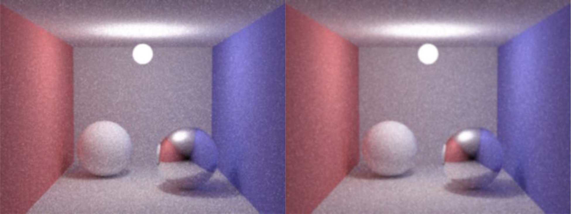
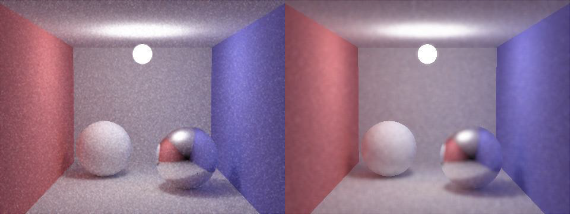
The object filters were a huge improvement over the simple filters in reducing noise while maintaining detail, but they fell short when preserving detail on specular surfaces. This is because the filters only take into consideration the object belonging to the pixel and not the object belonging to the reflection vector. My solution to this problem was to build upon the object filters; the filters would check if the surface is specular. If so, the filter would only be applied across those pixels whose reflection vectors belonged to the same object. Otherwise, the object filter would be applied as normal.

The first of the BRDF filters is the mean function. This function takes as input, the vector of pixel values, the vector of objects for which the pixels belong to, the vector of the objects for which the reflection vectors belong to (-1 if diffuse or no intersection) and the height and width of the image, and the kernel size. The filter applies an object based mean across the vector of pixel values as usual until it encounters a pixel belonging to a specular object.
When this happens, the filter, instead of considering pixels with the same object, only considers pixels with reflection vectors belonging to the same object. Then, the viable pixel values are averaged and applied to the center pixel. This method worked reasonably well in preserving reflection detail on specular surfaces.
The second BRDF based filter is the gaussian variation. This essentially works the same way as the BRDF mean; however it utilizes a weighted kernel with size specified by the user. When this method encounters a specular object, it applies the weights to only those pixels with reflection vectors belonging to the same object.
It continues to take the total of these weighted pixel values and divide by only those weights used. This value is then applied to the center, specular pixel. This method also worked well in maintaining the detail in specular objects.
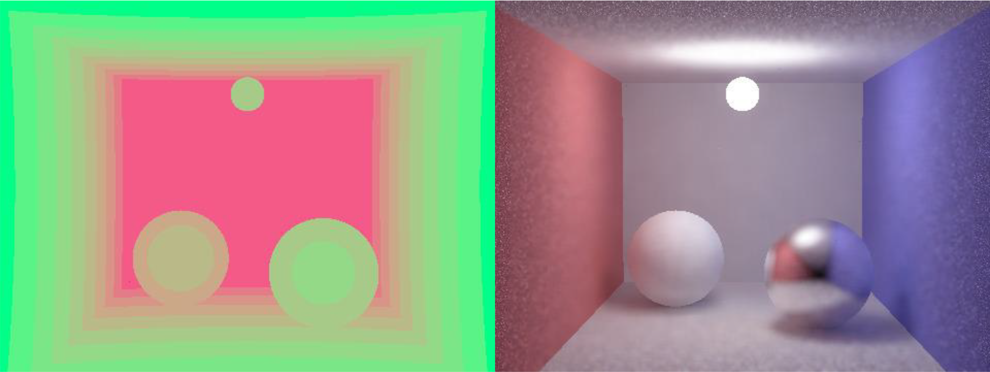
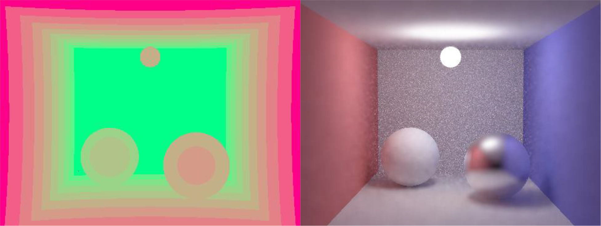
The next set of filters takes more information from the scene in an attempt to decrease the amount of noise in the renderings while preserving detail. The main idea behind these filters is that pixels with similar normal vectors should have similar pixel values. This is especially so in scenes with simple geometry. The following filters all take the pixel value vector, the object vector, the normal vector (normal value for each pixel), the height and width of the image and the size of the kernel to be applied.
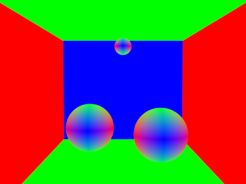
The normal mean filter takes a pixels neighbors and finds which pixels share the same object. Then, each of the neighboring pixels’ normal vectors are evaluated for their similarity with the center pixel’s normal value (dot product). These weights are then applied to each respective pixel value, totaled, then averaged (divided by the total weights). This final value is applied to the center pixel. This filter worked reasonably well in reducing overall noise while preserving detail.
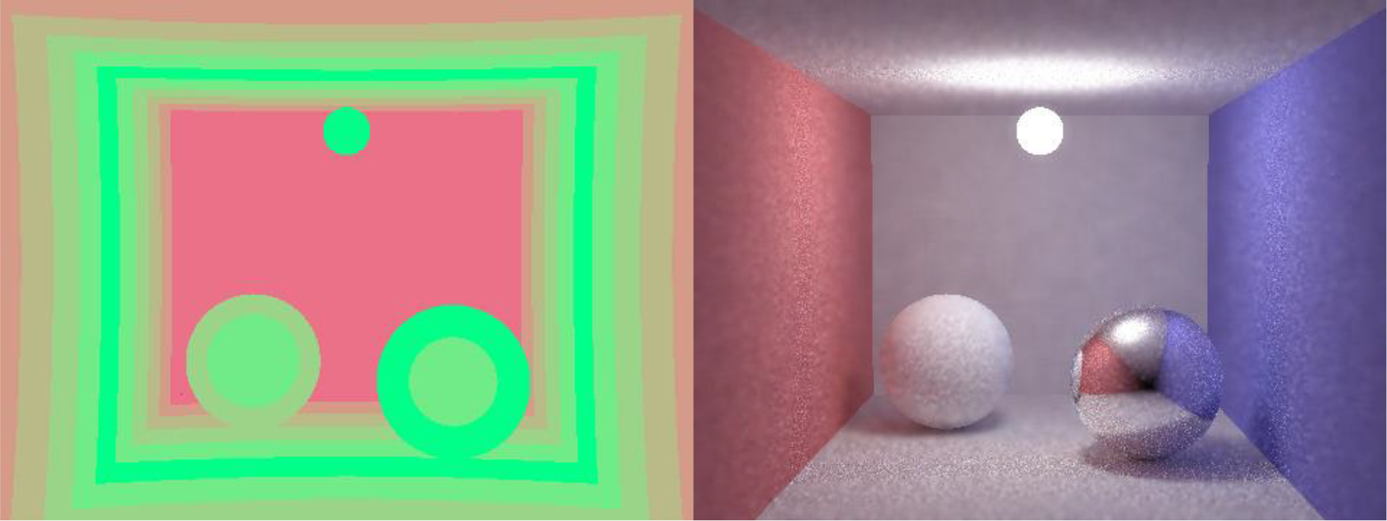
The normal gaussian variant constructs a gaussian kernel (weighted matrix) with the size determined by the user input. Then, each pixel in the neighborhood is assessed to see if it belongs to the same object as the center pixel. For each viable pixel, its normal is evaluated to see how similar it is to the center pixel’s normal vector.
These weights are multiplied by the weights in the kernel, and finally multiplied to the pixel values themselves. These weighted values are averaged and applied to the center pixel. This algorithm not only assumes that pixels with similar normal values should have similar values, but also that pixels closer to the center pixel should have more weight.
This method produced less impressive results than the normal mean filter, and removed overall noise in a reasonably acceptable fashion. The filter gives too much weight to the center pixels for it to work well on an image with this much noise.
The last variation of filter is the depth of field variation. The basic idea behind this filter is to use different sized filters for pixels at different distances. This filters takes as input the vector of pixel values, the vector of pixel object IDs, the vector of pixel depths, the height and width of the image, the number of levels of focus in the image, and the number of the level which should be in focus.
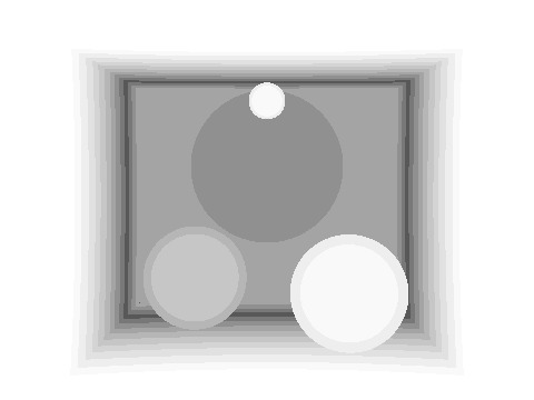
The DOF filter first computes the minimum and maximum pixel depths in the scene. From this, it bins the pixels according to their depth and the amount of levels specified by the client. From the designated focus level, the algorithm increments the filter size by two pixels for each level on either side of it.
For example, the pixels in the focus level are left alone. The pixels one level closer and one level further are subject to an object mean filter of size three. The pixels one level closer and further than those two levels are then subject to a filter of size five. The process continues until all pixels are filtered.
This filter produced interesting results but cannot really stand on its own for overall noise reduction. It would produce much more visually pleasing results when used in conjunction with other general noise reduction filters like the object median filter.
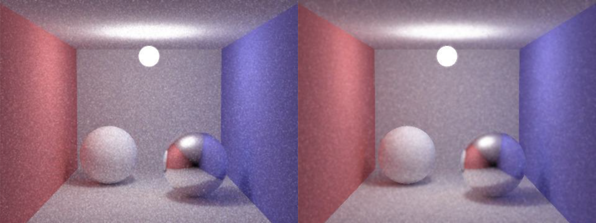
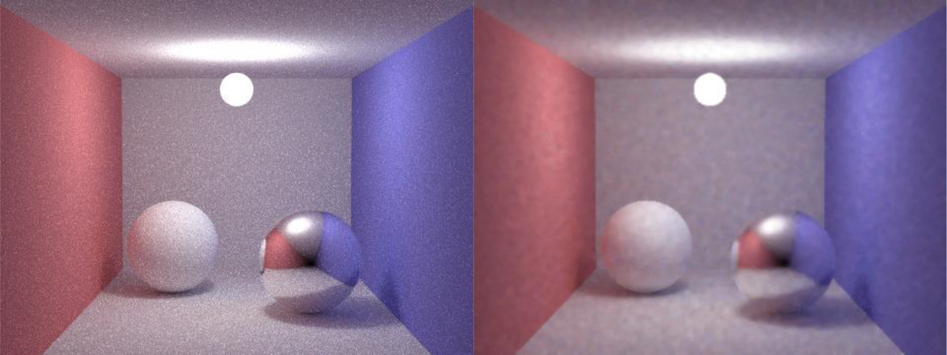
The main goal of these filters was to produce more visually pleasing results without increasing the amount of samples per pixels and therefore consuming less time. The filters were generally acceptable in their own right, but produced better results when combined. The combination which achieved the best overall results while taking least amount of time was applying an object median first (object specific aperiodic noise reduction) followed by a simple gaussian to reduce some of the aliasing introduced by the object based filter.
Monte Carlo ray tracing is a great technique when attempting to render realistic scenes. That being said, an inordinate amount of samples per pixel are required in order to produce results which aren’t completely riddled with noise. As it turns out, a number of post processing techniques can be implemented in order to reduce some of this noise without increasing the amount of samples per pixel.
Simple filters are very cheap in terms of time, but don’t utilize enough information about the scene in order to produce acceptable results on their own. Object based filters take a pixel’s object into consideration when applying each filter and produce acceptable results with little time overhead. BRDF filters further this concept by considering whether each pixel belongs to a specular object and incorporates the reflection vector’s object. Normal filters take another step in increasing the amount of information utilized by a filter; it considers the normal vector associated with each pixel and uses it as a weight in considering a pixel’s value. Finally, the DOF filter takes the depth of a pixel and applies different sized filters for different depths. This filter provides interesting results, but does little in the way of reducing overall noise.
The best function in terms of reducing general noise isn’t any one filter, but a combination of multiple filters. The combination which provided the best results with minimal time overhead was the object based median to remove aperiodic noise caused by under-sampling, followed by a simple gaussian filter to reduce some of the aliasing caused by the object based filter. This combination was able to produce similar results with time an order of magnitude less than those images produced with higher samples per pixel. With these results, I can conclude that post-processing can significantly reduce the amount of noise in Monte Carlo renderings while maintaining or improving upon both time complexity and visual fidelity.